My Little Projects

ML modelling

These are few examples of how ML can be used for predictions

Data is abundant now and is being collected constantly. Machine learning uses concepts of statistics and algorithms are written to see if any sense can be made of the data or if there is any pattern which can be learned. This learning can then be used to probably predict what the next data might be.
The data could be movies that someone loves to watch .Using a well-trained algorithm, one could make an educated guess on what the person might want to see next. The data could be images or even text /words that someone uses often in their emails or text messages.

Examples

Gazing at a Robin

Model a Successful campaign

Src: Photo by Tom Bradley on Unsplash

ML Model to make your campaign

Kickstarter is a crowdfunding platform with a community of more than 10 million people who are creative, tech enthusiasts.
Kickstarter works on all or nothing basis: a campaign is launched with a certain amount an artist or developer wants to raise. If it doesn’t meet its goal, the project owner gets nothing. For example: if a projects’ goal is $5000, even if it gets funded till $4999, the project won’t be a success.
If you have any project in mind to post to Kickstarter, the following classifier might help to predict the success of your project being funded or not.

The main steps that followed for building a predictive model are

Extracting data
Exploratory data analysis
Feature engineering
Building a model

This is an iterative process because data has to re-examined and model rebuilt after tuning the parameters and processing the features until the best fit is found. During this iterative process, one must not sacrifice the simplicity for complexity.

Exploratory Data Analysis

Understanding the data is very vital before moving on to classifying or evaluating it. This process is called Exploratory Data Analysis (EDA). This important step enables one to spot anomalies before beginning the Machine Learning model. It also brings out the bigger picture of the data. EDA could be done in a Graphical or Non-Graphical means. Non-Graphical methods are generally the summary statistics. EDA could also include methods to

Reduce Dimensionality: Reduce the number of features to a linear combination of data so that data has fewer features (Columns) which can explain most of the variance.
Analyse the Cluster: Data can be organised into clusters so that similar observations are clubbed into clusters.

Reading and uploading data

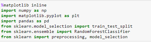
Python is the languaged used to analyse and build the model.The following libraries are imported

pandas: for easy manipulation of data structures.
NumPy: For scientific computations
sklearn : The machine learning library of Python

The data used for this evaluation has been downloaded and stored as a stored as a CSV file which is the commonly used format for exchanging data. To begin with, read the CSV file into a variable.

To build a model, the projects that have already been evaluated have to be studied. In order to do that we divide the whole raw data into two data frames. One of which to used to model the prediction model and the other to test if our model is accurate. The variable /column named ‘Evaluation_set’ is used to identify if the project has been evaluated or not. The Data Frame named ‘modelling_df’ will be is used to build the model.

Check Context of data

The dataframe which is used for modelling has 50,000 instances or sample projects and 27 features or columns describing various details about the project. The target is the column named ‘State’ which is either a 1 or 0 based on if the campaign was successful/unsuccessful.

Out of the 27 columns/features the data types of the features have to be checked. A check needs to done to see how many have valid values in them.

Most of the columns are numerical but a few are non-numerical. Since an ML model cannot be built on non-numerical column one needs to now study on how the columns can be made numerical or eliminated altogether. The feature named ‘ Country’ describes which country the project belongs to. There are a few unique values. It is definitely a categorical column.

Check for null values and fetaures having single value or outliers

There are many columns which have many nulls or values which predominantly have only one value or many outliers. An initial check could be made to see which columns to retain and columns that could be dropped. This can be done using statically data or graphically plotting the values The above function is used to check the distinct value counts, nulls, mean, standard deviation etc of all the columns and decision can be taken on what columns could be retained.

Preprocessing

Machine learning algorithms require inputs to be numerical and so if there are any columns which are categorical, they need to somehow be transformed into numerical before using them to predict a model. One of the common ways to handle categorical columns is ‘One Hot Encoding’. This technique can be employed when the values have no particular ordering. For every unique value of the column , another column is created where the value is 1 if for that instance the feature takes that value else 0. For example, the column ‘country’ could be the US. So, a new column (Country_US) can be created which will have a value 1 or 0 based on if the value of the column is ‘US’ or not. We could use a column transformer to convert all the categorical columns but since we have only one column named ‘Country’ we could use a function.

Dropping columns ahve redundant or missing data

The features - currency symbol, trailing code and currency can be dropped. The features ‘is_backing’, ‘permissions’, ‘friends’ and ‘is_starred’ have many missing values, so they could also be dropped at this moment. The column ‘URLs’ and ‘source_url’ contain only URLs and modelling algorithm needs numeric data, so they could be dropped. There are a few columns which are JSON string which has to be looked in separately to extract only the columns which add value to the modelling. The columns to be retained are identified and a new data frame created containing only the columns to be retained.

Reduction of the feature set

Some of the columns are redundant and some of them can be clubbed to become one column. To compare the various projects, it would be better to convert the ‘money to be raised’ to a single currency. Since the USD rate is given for the various currencies, a new column is created ‘goal_in_usd’.

To make sense of the dates we could club the various dates and create single columns containing the various duration in milliseconds.

Some of the columns from the multiple columns stored in the JSON string can be extracted and added the data frame on which modelling is performed. Looking at the ‘category’ column, the value of column ‘slug’ could be split to obtain the ‘parent category’ and the ‘category column’. These columns are categorical columns so they could be encoded too.

Scaling

From the data, it is very obvious that the columns have various units. In some machine learning algorithms, the units have to be scaled because certain weights may update faster than others. Algorithms like Decision tree or k-nearest neighbours are not affected by the scaling. There are a few methods which can be used to scale features. Some of them are the StandardScaler, MinMaxScaler, RobustScaler and Normalizer. MinMaxScaler is used in this case and it follows the following formulae

The range of the features is now shrunk to values between 0 and 1. If there were negative values the scaler shrinks them to values between 1 and -1. However, this scaler is sensitive to outliers.

After the first round of preprocessing, we have 169 columns.

All columns are scaled between 0 and 1.
Category columns have been one hot encoded
All datetime columns have been transformed so that we have logical columns which contain some period in seconds.
Columns which have more than 50% as null values or missing values are dropped.
All objects which are non-numerical and irrelevant at this stage are dropped.
No custom transformations have been applied.

Modelling

There are many algorithms that can be used. Since this project requires a prediction on the state of the project which is either a 1 or 0(Successful/ Unsuccessful), it is considered as a classification problem. Logistic Regression and Decision Tree are two good models to build and test.

DECISION TREE

The decision tree is the first model that will be fitted. The data is divided into smaller datasets based on a certain features until the target variable (‘State’) falls in one of the 2 categories (0,1) GridSearch is used so that the hyperparameters can be tuned to get the most optimal value for the model. The GridSearchCV of the sklearn library is used. A cross-validation process is performed for achieving better results. In K-Fold cross-validation, a given dataset is split into K number of folds or sections. Each of the K folds is considered as testing set at different iterations. For this modelling, we have used 5 fold cross-validation. The best combination of the hyperparameters is chosen.

The results are sorted based on the scores of the test and the best combination is picked. The table below displays the results and it is clear that the ‘max depth’ of 13 gives the best accuracy

We could have a look at the features which play an important part in this model.

It can be seen that profile_state and Goal_in USD are 2 columns which have the most influence. One can also see the categories and subcategories which are highly influential.

LOGISTIC REGRESSION

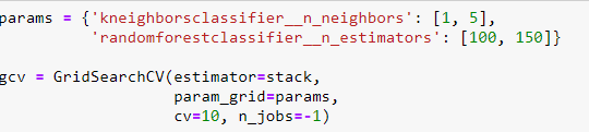
Similar to the Decision Tree, we build a Logistic Regression model too. We use GridSearch and provide certain hyperparameters and chose the combination which gives the best result

As can be seen from the results, the best results are for a value of C = 4

Logistic Regression seems to give better results than the Decision tree, though the accuracy is only 76%. We could further preprocess by applying a PCA of the columns which have very high variance. We could extract more columns and scale them using another scaler. The process of preprocessing and hyper tuning the parameters is an iterative process. Care has to taken not to overfit the model.

To view the whole code please use the link Kickstarter
To improve the results of the Machine learning solution one can

Try different algorithms
Look into features that can be used/dropped and feature engineering
Tune the hyperparameters of the algorithm selected.

ML Model to detect Parkinsons

Parkinsons is a nuerodegerative disorder in which a part of the brain gets damaged progressively over years.
More than 1 million people in UK are affected by Parkinsons. People suffering from Parkinson's have not enough dopamine because the nerve cells producing them have been damaged.

The main steps that are followed for building a predictive model are

Extracting data
Exploratory data analysis
Feature engineering
Building a baseline model
Building different models
Comparing the metrics to check if model gives best result

Main Objective

To build a model which can accurately detect if a person has PD (parkinson's) or not. The dataset used is from UCI ( Center for Machine Learning and Intelligent Systems). The dataset was created by Max Little of the University of Oxford, in collaboration with the National Centre for Voice and Speech, Denver, Colorado, who recorded the speech signals of many PD patients. Use this link to download the data and learn further details The data consistes of voice recordings of 31 people out of which 23 are Parkinson's patients. The dataset is composed of a range of biomedical voice measurements. Each column in the table is a particular voice measure, and each row corresponds one of 195 voice recording from these individuals ("name" column). The main aim of the data is to discriminate healthy people from those with PD, according to "status" column which is set to 0 for healthy and 1 for PD.

Information of the features

Attribute Information:

Matrix column entries (attributes):
name - ASCII subject name and recording number
MDVP:Fo(Hz) - Average vocal fundamental frequency
MDVP:Fhi(Hz) - Maximum vocal fundamental frequency
MDVP:Flo(Hz) - Minimum vocal fundamental frequency
MDVP:Jitter(%),MDVP:Jitter(Abs),MDVP:RAP,MDVP:PPQ,Jitter:DDP - Several measures of variation in fundamental frequency
MDVP:Shimmer,MDVP:Shimmer(dB),Shimmer:APQ3,Shimmer:APQ5,MDVP:APQ,Shimmer:DDA - Several measures of variation in amplitude
NHR,HNR - Two measures of ratio of noise to tonal components in the voice
status - Health status of the subject (one) - Parkinson's, (zero) - healthy
RPDE,D2 - Two nonlinear dynamical complexity measures
DFA - Signal fractal scaling exponent
spread1,spread2,PPE - Three nonlinear measures of fundamental frequency variation

Reading and uploading data

Python is the languaged used to analyse and build the model.The following libraries are imported

pandas: for easy manipulation of data structures.
NumPy: For scientific computations
sklearn : The machine learning library of Python
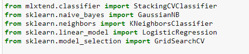
xgboost : To create a Boosting Model
mlxtend :The library for builiding a stacking classifier
matplotlib : Plotting graphs od data and results to visualise and understand better

The data used for this evaluation is stored as a CSV file format. It does contain a header and comma is used to seperate the various features. To begin with, read the CSV file and convert the data into a pandas dataframe.

The data is inspected.The various features/attributes is inspected. There are 24 columns. The column 'name' which is used to identify the patient adds no value in training the model. The column named 'status' is the target which we need to predict. It can have 2 values '1' if the patient has PD, 0 if healthy. So we could assign 'y', the target pandas series as the column 'status'. All the columns except 'name' could be assigned to 'X'.

Feature Engineering

There are no columns with categorical values . So there is no need to One-hot encode or label encode any feature.
The features have varying minimum and maximum values. The reason could be that the features have different magnitude or units. Most of the ML models are not interested in the units or magnitude .Obviously, the features with higher magnitude might weigh more than thoses with lesser magnitude. If we are to use algorithms which computes distance between feature point then scaling is a must.K-Nearest neigbhors is sensitive to the distance between feature points where as Tree-based models do not care about the distance.
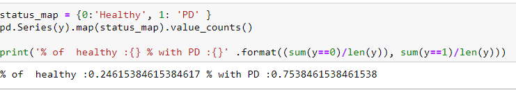
Upon inspecting the 'status column it can be noticed that there is a imbalance in the distribution of values. 75% of the people observed have PD wheare as 25% are marked as healthy. There is a slight class imbalance. Care must taken to ensure that a healthy person is not misclassified as 'PD' since the status value '1'(PD) is the dominant class. This causes unecessary heartache for a healthy patient as well as the model will become unrealiable. Since PD is not a minority class, wrong classification will not cost a life.
lib

'Accuracy' cannot be used as the scoring strategy in this case. We could oversampling the minority class but that might lead to overfitting. Undersampling the majority class might lead to model being biased. The ROC AUC scores could be used to compare and select a model.The ROC curve evaluates the probablity predictions made by the model on the test dataset. It is a plot of the flase-positive rate to the true positive rate.Thus helps to undertand the tradeoffs. Geometric-Mean or G-mean could also be used as a mteric to seek the balance between sensitivity and specificity.Precision-Recall curve couls also be used to check the performance of the classifier on the positive class.
The hyperparameter 'class-weight' is set as 'balanced' so that less weight is put on the majority class
n_samples/ (n_calss *np.bincount(y))

Split the data

The data is generallly split into training and testing sets. Around 20% is set aside as test data.

Baseline Model

Let us consdier to first use Logistic regression as the classifier to create a baseline model. This is not optimised and will be used to compare with other models.

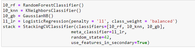
Ensemble Model

When several ML techniques are combined together it is called as ensemble and this improves the accuravy of the predictions sometimes. They are combined to reduce the variance(bagging), bias(boosting) and predictions accuracy(stacking).
Ensemble models are grouped as sequential or parallel. If the base learners are generated sequentially and each learns from the previous models it s grouped as sequential.The weghts of the mislabbelled instances are boosted so that the next sequenetial model learns from it. In parallel, the base learners are independent of each other. Bt averaging, the errors are reduced.

Bagging

Bagging stands for Bootstarp aggregating. Bootstarp samples are used to obtain various data susets to train the base learners. By avaraging the multiple estimates from the various base learners ,the overall variance of the estimate is reduced.
Random forest is one of the common algorith in ensemble. Instead of using all the features, a random subset of features is selectes , thus further randomising the tree. Though bias might increase, the variance is decreased.

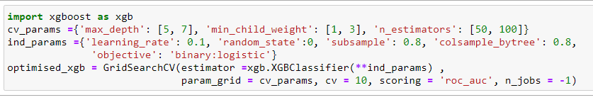
Boosting

Several weak learners are better than random guessing. The misclassified instances are given more weight and trained again. Finally the weighted sum or weighted majority vote is used to decide on the final prediction

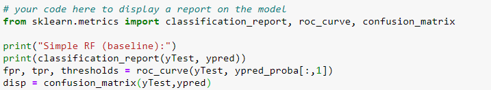
Comparing the models

Since there is a slight class imbalance, Classification report or accuracy score is not the metrics to be used to compare this models. This is a binary classification having labels as 0 or 1 . The default threshold for the probablity is 0.5. The value of probablities less than the threshold of 0.5 are assigned to class 0 and values greater than or equal to 0.5 are assigned to class 1. The class distribution for this dataset is slightly skewed and the cost of one type of misclassification is more important than another type of misclassification. So the optimal threshold has to be chosen. 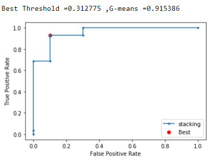ROC curves can be used to analyse the predicted probablities of the model and the ROC-AUC curves could be used to select the best model. The curve gives an picture of the true and fale positive rates for the various thresholds.The area under the curve gives the accuracy of the model. 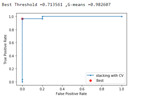If we adopt the boosting model then the optimum threshold could be set as 0.71

prediction < 0.71 = Class 0
prediction >= 0.71 = Class 1

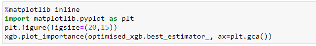
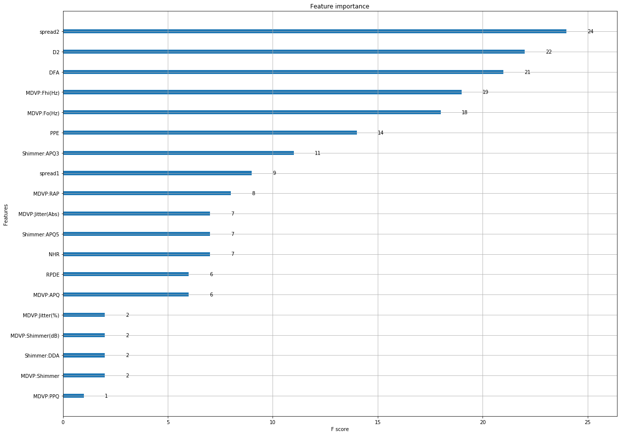
Understanding the importance of the features

Since Boosting seems to give the best score, if we decide to using a boosting model, xgboost classifier is able to show which attributes where considered important by the model A plot of the importances of features with weights for each feature is displayed .The weights sum to one.